Research Article

Impact of Livestock and Fisheries on Economic Growth: An Empirical Analysis from Pakistan

Farrukh Ilyas1, Durdana Qaiser Gillani2, Mudassar Yasin3, Muhammad Amjed Iqbal4, Iqbal Javed5*, Shahbaz Ahmad6 and Iftikhar Nabi7

1Department of Economics, The University of Punjab, Lahore, Pakistan; 2Department of Economics, University of Lahore, Pakistan; 3Department of Agricultural Extension, MNS-University of Agriculture, Multan, Pakistan; 4Institute of Agricultural and Resource Economics, University of Agriculture, Faisalabad, Pakistan; 5Department of Economics, University of Lahore, Sargodha Campus, Sargodha, Pakistan; 6Department of Education, University of Lahore, Sargodha Campus, Sargodha, Pakistan; 7Agricultural Economics Section, Ayub Agricultural Research Institute, Faisalabad, Pakistan.

Received | August 04, 2021; Accepted | July 07, 2021; Published | November 30, 2021

*Correspondence | Iqbal Javed, Department of Economics, University of Lahore, Sargodha Campus, Sargodha, Pakistan; Email: iqbaljaved_uaf@hotmail.com

Citation | Ilyas, F., D.Q. Gillani, M. Yasin, M.A. Iqbal, I. Javed, S. Ahmad and I. Nabi. 2022. Impact of livestock and fisheries on economic growth: an empirical analysis from Pakistan. Sarhad Journal of Agriculture, 38(1): 160-169.

DOI | https://dx.doi.org/10.17582/journal.sja/2022/38.1.160.169

Keywords | Economic growth, Gross capital formation, Livestock, Fisheries, Pakistan

Introduction

The development of economies and their economic growth also depend on agricultural development. A great deal of literature has argued that agricultural development is a cause of the economic transformation of a country as a whole. For industrialization processes, the contribution of raw materials as inputs by the agricultural sector is very essential. For poor countries, economic growth is based on the growth of agricultural sector. In the history of development of England, the agriculture sector played a vital in the industrialization of the country. So, the economic development and growth of a country in all aspects is possible by agricultural development (Tsakok and Gardener, 2007). Over the years, it has been observed that the share contributed by agriculture sector in Gross Domestic Product is reducing. The rural population proportion is also declining as people are migrating to urban areas for better opportunities and facilities available in urban areas. Despite an increase in global agricultural trade volume, the trade structure is hanging considerably over the past decade. The high-value products (i.e., fishery and vegetables) have increased their contribution to the global trade volume. The developing countries have also observed a tremendous enhancement in these high-value exports which caused a decline in the export of their traditional products like coffee, cocoa, and tea. So the developing countries need to focus their analysis on these high-value trade products such as vegetables, fruits, fish, and their processed products which form fifty percent of the export volume of these countries. There has been observed an increase in agricultural productivity in most developing regions except in Sub-Saharan Africa and South Asia (Meijerink and Roza, 2007).

Agriculture sector has been contributing very well to the economy of Pakistan since its creation. The population census of Pakistan 2017 reveals that about 60% population of Pakistan lives in rural areas. So the agriculture sector is a source of income for the majority of population. According to Pakistan Bureau of Statistics, agriculture absorbs half of the labor force and provides foreign exchange for Pakistan. Livestock also acts as a substitute of insurance for poor households as it can be sold in the time of severe difficulty (Islam et al., 2016). Its contribution to Gross Domestic Product is 24 percent. According to Lopez et al. (2017), the agricultural industry has a ripple effect on the economy as it purchases services, agricultural equipment and inputs from other sectors contributing to the growth of those sectors of the economy as well. Farming also creates short term contractual jobs in the electrical works, engineering and labor market. Today not only farms but also livestock, poultry and fisheries are important components of agriculture sector contributing a major share in the Gross Domestic Product of the country with an increase in the demand for meat, eggs, dairy products and related goods due to an increase in population.

Agriculture sector is comprised of many sub-sectors. The major sub-sectors that have significant effects on the agricultural output are such as crops, livestock and poultry, forestry and fisheries. All these sectors play some vital role in the economy by providing employment opportunities and acting as a source of income for many poor and marginal households. In this way, agricultural subsectors enhance economic development. Livestock enhances the rural socio-economic development of Pakistan. It is comprised of cows, buffalos, goats, camels, horses, and donkeys. Livestock production activities provide more than 35 percent income to about 8 million families involved in raising livestock. The rural poor also get their livelihood from livestock raising and it is considered as a source for their survival. So it is playing a crucial role in poverty alleviation. The contribution of livestock to the agriculture value added is 58.3 percent approximately and 11.4 percent to the overall Gross Domestic Product during 2016-17 (GoP, 2017). With the growth in the world economy and trade, the share of fisheries is increasing in the world food. The increase in the quantity of exports of fish and fish products is 12.20 percent and the increase in value of fisheries is 15.09 percent during 2016-17. The fisheries departments are doing much in introducing fishing methodologies, developing value-added products, enhancing per capita fish consumption and uplifting the living standard of fishermen (GoP, 2017).

Here, we review the studies showing the importance of sectors in the economic growth of developing as well as developed countries. Vogel (1994) analyzed the multiplier effects of agriculture using cross-section regressions. The social accounting matrix multiplier is used to run the cross-section regression by using the data set of 27 countries. Vogel has conducted this research to study the forward and backward linkages created by agricultural development. The results reveal that agriculture is a great source of economic growth for all 27 countries in the early stages of growth but as the countries move towards industrialization their growth starts slowing down. Gollin et al. (2002) used a structural transformation model based on the neoclassical growth model to check how agriculture sector affects economic growth. The results show that the agricultural productivity growth contributes a lot to the growth of the selected developing countries. Moreover, low growth in agricultural productivity can slow down the process of industrialization causing the per capita income growth to fall quite behind the developed countries. Fisheries have a direct and indirect effect on economic activity (Murray, 2014). Fisheries also contribute a significant part in generating employment and contributing to the output of the region. Enu (2014) has analyzed the impact of fisheries on growth. The regression results show that crops/livestock increases Gross Domestic Product growth but it is insignificant in case of Ghana. Chongela (2015) analyzed the impact of agriculture on Tanzanian economy growth. The multiple regression model is estimated to see the impact of agriculture sub-sectors (crops, livestock and fisheries) on the agricultural Gross Domestic Product. The results of multiple regression show that sub-sectors significantly affect the agricultural Gross Domestic Product. So, economic activity can be enhanced by promoting the sub-sectors of agriculture. Javed et al. (2018) find the determinants of the economic growth of Pakistan by using different variables. The impact of population and imports of Pakistan is found positive, while the impact of inflation and democracy was negative. The impact of education spending, exports and foreign direct investment are insignificant. Fatima et al. (2019) conducted research on Pakistan’s bilateral trade and find that the product of Gross Domestic Product, trade to Gross Domestic Product ratio and population of Pakistan has a positive and significant effect on Pakistan’s bilateral trade with major trading partners. The results suggest that Pakistan’s exports mostly depend on agriculture and needs to concentrate more on improving trade relations with those countries which have cultural similarities and joint borders. Improvement in managing Pakistan’s marine fisheries can improve economic growth and resource sustainability (Kaczan and Patil, 2020).

Awan and Alam (2015) show that agricultural productivity enhances economic growth on the basis of data from 1972 to 2012 in Pakistan economy. It is found that agriculture value addition significantly affects economic growth. Trade openness, gross capital formation and employed labor force also positively affect economic growth. Moreover, inflation affects economic growth negatively. Engida et al. (2015) use modified recursive dynamic extension of the Computable General Equilibrium model introduced by the Internal Food Policy Research Institute. The results reveal that growth in livestock sector can cause growth in overall Gross Domestic Product and agricultural value-added as well. The accelerated productivity in livestock can also increase the efficiency of other related sectors. Ibrahim et al. (2017) showed that farming and livestock affect economic development. The result shows that there exists a positive relationship between farming and economic development. Secondly, the correlation between livestock production and economic growth is tested and the results show an association between the two variables. The regression analysis shows that both farming and livestock positively affect the economic development of Mogadishu.

Considering the role of agriculture in the economy, many studies had been done to check how the agriculture sector affects economic growth. A quite number of studies are found in the literature that investigated this impact. Most of the studies show that agriculture and its sub-sectors positively affect economic growth and they also create employment and income opportunities in the economy of the country. Agriculture plays an important role in the economy of Pakistan but this study is conducted to estimate the impact of only fisheries on the economic growth of Pakistan so that proper policies could be recommended for the growth of the fisheries sector to be in line with the economic growth of Pakistan. But a little literature is found on the separate effect of agricultural sub-sectors on economic growth. This study emphasizes to analyze the effect of livestock/poultry and fisheries on the economic growth of Pakistan which will be a significant contribution in the existing literature.

Matrials and Methods

On the basis of available literature and empirical work, the following model has been developed to check the influence of livestock and fisheries on the economic growth of Pakistan.

(1)

GDP: GDP per capita in constant LCU; MIC: Minor crops value addition in agriculture (percentage); MAC: Major crops value addition in agriculture (percentage); LIVS: Livestock value addition in agriculture (percentage); FISH: Fisheries value addition in agriculture (percentage); GCF: Gross capital formation as GDP (percentage); t: time.

The econometric form of the equation written above can be as follows:

……..(2)

βo is the intercept of the equation and βi are coefficients of the explanatory variables where µt is the error term of the model.

The research aims at investigating the impact of sub-sectors of agriculture (livestock and fisheries) on economic growth of economy. Major crops, minor crops and gross capital formation have been used as control variables. The data from 1987 to 2017 has been used which is extracted from different Economic Surveys of Pakistan.

Nelson and Plosser (1982) highlight that most of the time series data is non-stationary which makes the regression results spurious. So to avoid spurious results, we have used Augmented Dickey-Fuller test to identify the problem of non-stationarity of time series data. ADF test has the following general forms:

(without constant and time trend) ……..(3)

(with constant and no time trend) ……..(4)

(with constant and time trend) ……..(5)

Where;

Yt is any time series to be tested for unit root, t shows time trend and et is residual with white noise properties and Yt-j denotes the lagged values of the variable under study. If lag j=0, simple Dickey Fuller test will be applied for testing unit root. The following are the null and alternate hypothesis for ADF unit root test:

H0: δ= 0 (the time series has a unit root)

H1: δ<0 (the time series is stationary)

The null hypothesis is tested by estimating the coefficient of Yt-1 using OLS and the τ -statistic is computed which is compared with the critical τ -value of Dickey Fuller (1979).

Johansen multivariate co-integration technique is used to show the log-run associations of variables equation (2) as the time series under study are non-stationary. The Johansen co-integration method is based on Vector Auto Regressive (VAR) model with k lags which is as follows:

(6)

Yt is the vector of variable stationery at the first difference that is I(1); βi are the parameters and ut is white noise error term.

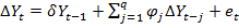
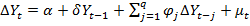
The presumption of co-integration is that there exists at least unidirectional causality among variables which is determined by Vector Error Correction Mechanism. The simplest equation of the Vector Error Correction Model is given below:

...(7)

Where and

The matrix π is crucial in Johansen co-integration as it contains the long-run coefficients. This is also called as a reduced rank matrix as its rank is always less than the variables in the equation. If r is the rank and k is number of variables than r < k.

Results and Discussion

The descriptive statistics give the temporal properties of the data as shown in Table 1. The results reveal that log of Gross Domestic Product and minor crops are positively skewed whereas major crops, livestock, fisheries and gross capital formation are negatively skewed. The variables also have kurtosis as all variables have values less than 3. But the results are insignificant. Jarque-Bera shows that all the variables of the econometric model are normally distributed with zero mean and constant variance, so we conclude that data sets are normally distributed.

We apply Augmented Dickey Fuller unit root test to check the presence (absence) of unit root in the series. Table 2 contains Augmented Dickey Fuller unit root test which shows that log GDP and GCF are stationary at first difference at 5% level of significance. However, variables such as MIC, MAC, LVS, and FIS are stationary at the first difference at 1% level of significance. Since all variables are I(1) so Johansen co-integration approach will be applicable for long run association of variables.

Lag length criteria

For lag order, Vector Auto Regressive approach has been used allowing two lags for estimating the lags of variables to be used for co-integration. Table 3 shows the results of Vector Auto Regressive. Likelihood Ratio, Final Prediction Error, Akaike Information Criteria and Hannan Quinn suggest using 2 lags whereas Schwarz Criterion suggests 1 lag. In the study, 2 lags have been used for the co-integration approach.

 

Table 1: Descriptive statistics.

	LOG-GDP	MIC	MAC	LIVS	FISH	GCF
Mean	4.670117	0.148378	0.336138	0.475763	0.022793	17.50514
Median	4.644791	0.148695	0.341422	0.479321	0.022905	17.71120
Maximum	4.791220	0.195237	0.444237	0.597252	0.032020	20.81826
Minimum	4.550300	0.112951	0.242563	0.343291	0.013326	14.12063
Std. Dev.	0.069733	0.023574	0.068690	0.083796	0.005013	1.814580
Skewness	0.120873	0.201807	-0.076912	-0.082749	-0.315067	-0.172707
Kurtosis	1.758818	1.875704	1.450365	1.583181	2.379028	1.892441
Jarque-Bera	2.065343	1.843139	3.132331	2.628239	1.010953	1.738580
Probability	0.356054	0.397894	0.208844	0.268711	0.603218	0.419249
Sum	144.7736	4.599720	10.42027	14.74864	0.706585	542.6594
Sum Sq. Dev.	0.145880	0.016672	0.141551	0.210655	0.000754	98.78098
Observations	31	31	31	31	31	31

 

Table 2: Augmented dickey-fuller unit root test.

Variables	Level	First Difference
	τ -statistic	τ -statistic
LogGDP	0.0757	-3.0967**
MIC	-0.7246	-5.1155*
MAC	-0.6582	-5.1512*
LVS	-0.4248	-5.9753*
FIS	-1.8776	-3.9671*
GCF	-1.3417	-3.6068**

Critical Values at Level: *1% = -3.6793; **5% = -2.9678; ***10% = -2.623; Critical Values at 1st △: *1% = -3.6892; **5% = -2.9719; ***10% = -2.6251

 

Empirical analysis

Since variables are non-stationary of the same order, so Johansen co-integration approach is applied to determine the long-run relationship of variables (if any) based on Vector Auto Regressive which is sensitive to lags used, a great deal of time has been spent for selecting the lag length. The lag length of 2 has been used as per Akaike Information Criteria which will help to decrease the degree of autocorrelation in the model.

Johansen co-integration approach uses two likelihood ratios for testing the null hypothesis. The two likelihood ratios are trace and maximum Eigen likelihood ratios. Table 4 and 5 highlight trace and maximum Eigen statistic results respectively. Both trace and maximum Eigen statistics reject the null hypothesis at 5% critical level and indicate that there exist three co-integrating vectors recognizing relationship of variables.

 

Table 3: VAR lag order selection criteria.

Lag	LogL	LR	FPE	AIC	SC	HQ
0	393.6596	NA	9.87e-20	-26.73514	-26.45225	-26.64655
1	527.1079	202.4733	1.26e-22	-33.45572	-31.47549*	-32.83554
2	582.3616	60.96961*	4.76e-23*	-34.78356*	-31.10600	-33.63179*

(*) show lag order at 5% critical level; AIC and SC: Akaike and Schawarz information criterion.

 

Table 4: Joahnsen cointegration rank test (Trace).

Hypothesized No. of CE(s)	Eigenvalue	Trace Statistic	0.05 Critical Value	Prob.**
None*	0.960509	209.2066	95.7536	0.000
At most 1*	0.890414	118.7196	69.8188	0.000
At most 2*	0.631778	56.81032	47.8561	0.0058
At most 3	0.409485	28.83635	29.7970	0.0642
At most 4	0.339009	14.08706	15.4947	0.0806
At most 5	0.085241	2.494658	3.84146	0.1142

Trace test indicates 3 cointegrating eqn(s) at 0.05 level

 

Table 5: Johansen cointegration rank test.

Hypothesized No. of CE(s)	Eigen value	Max-Eigen Statistic	0.05 Critical Value	Prob.**
None*	0.960509	90.48698	40.0775	0.000
At most 1*	0.890414	61.90931	33.8768	0.000
At most 2*	0.631778	27.97397	27.5843	0.0446
At most 3	0.409485	14.74929	21.1316	0.3068
At most 4	0.339009	11.59241	14.2646	0.1269
At most 5	0.085241	2.494658	3.84146	0.1142

Max-eigenvalue test indicates 3 cointegratingeqn(s) at 0.05 level

 

Table 6: Normalized co-integrating coefficients.

LOGPCY	MIC	MAC	LIVS	FISH	GCF
1.000000	-0.587241	-1.654011	-2.530671	-4.701063	-0.009361
S.E	(0.08214)	(0.05786)	(0.06052)	(0.13534)	(0.00029)
τ -value	-7.14927	-28.58643	-41.81543	-34.73521	-32.27931

 

Long-rung relationship

Table 6 shows the normalized co-integrating coefficients after normalizing the first co-integrating vector Log Gross Domestic Product.

The following equation given below is the final normalized equation for a long-run relationship among the variables.

Log GDP = 0.5872 MIC + 1.65401 MAC + 2.5307 LIVS + 4.7011 FISH + 0.00936 GCF

The first normalized equation of co-integration depicts that livestock positively affects Gross Domestic Product. A 1% increase in value addition of livestock will increase the Gross Domestic Product by 2.53% as this sector also has a good share in exports of Pakistan.

The fisheries sub-sector also affects the per capita Gross Domestic Product positively. 1% increase in the value addition of fisheries will increase per capita Gross Domestic Product of Pakistan by 4.7%. Other variables which are minor crops, major crops and gross capital positively affect the per capita Gross Domestic Product.

Short-run vector error correction model results

Vector Error Correction Model has been used to determine the short-run dynamics of the model. Table 7 shows the results of Vector Error Correction Model. The results show that most of the variables have a negative and insignificant impact on the GDP. The co-integration coefficient of the first equation has a negative value which shows that there has been an adjustment in disequilibrium in the period of study. The coefficient of adjustment is negative and significant which depicts that the log Gross Domestic Product adjusts towards equilibrium path by 77.96% in one year so it is going to take approximately (1/0.779637 = )1.28 years for Gross Domestic Product per capita to return to its equilibrium path which is a speedy adjustment. The Vector Error Correction Mechanism model is as follows:

Log PCY =- 0.003 + 1.717 Log GDP(-1) + 0.133 Log GDP(-2) + 0.064 MIC(-1) – 0.998 MIC(-2) – 0.308 MAC(-1) – 0.649 MAC(-2) – 0.598 LIVS(-1) – 0.959 LIVS(-2) – 2.336 FISH(-1) – 0.391 Fs(-2) – 0.004 GCF(-1) – 0.003 GCF(-2) – 0.7796 VECM(-1)

Diagnostic test results

The results of Diagnostic Tests are shown in Table 8. Jarque-Bera normality test shows that errors are normally distributed with zero mean and constant variance. Breusch-Godfrey LM based test for auto-correlation shows no auto-correlation.

White test to check for hetroskedasticity shows that the model does not contain hetroskedasticity problem that is the variance of the error terms is constant. Ramsey RESET test shows that the model does not contain misspecification.

Parameter’s Stability Test: Cumulative Sum (CUSUM) and Cumulative Sum of Squares (CUSUMSQ) tests show stability of the model. Figure 1

 

Table 7: Vector error correction estimates.

Error Correction:	D(LOGPCY)	D(MIC)	D(MC)	D(LS)	D(FS)	D(GCF)
CointEq1	-0.779637	-0.954459	-2.326618	2.804529	0.128280	1.577258
	(0.33551)	(0.34151)	(1.19423)	(0.81692)	(0.12167)	(50.9070)
	[-2.32377]	[-2.79485]	[-1.94821]	[ 3.43305]	[ 1.05433]	[ 0.03098]
D(LOGPCY(-1))	1.716999	1.778548	2.790735	-3.784055	-0.045609	100.3594
	(0.54576)	(0.55552)	(1.94264)	(1.32888)	(0.19792)	(82.8098)
	[ 3.14605]	[ 3.20156]	[ 1.43657]	[-2.84756]	[-0.23044]	[ 1.21193]
D(LOGPCY(-2))	0.132959	0.614008	0.735654	-0.996169	0.019967	41.61111
	(0.37218)	(0.37884)	(1.32478)	(0.90622)	(0.13497)	(56.4718)
	[ 0.35724]	[ 1.62077]	[ 0.55530]	[-1.09926]	[ 0.14793]	[ 0.73685]
D(MIC(-1))	0.063509	-0.818566	-1.242549	1.697841	0.113066	18.03844
	(0.44067)	(0.44855)	(1.56855)	(1.07298)	(0.15981)	(66.8632)
	[ 0.14412]	[-1.82493]	[-0.79217]	[ 1.58237]	[ 0.70752]	[ 0.26978]
D(MIC(-2))	-0.998288	-0.716054	-1.331909	1.503662	0.234745	-60.07732
	(0.50877)	(0.51787)	(1.81096)	(1.23880)	(0.18450)	(77.1966)
	[-1.96217]	[-1.38269]	[-0.73547]	[ 1.21381]	[ 1.27231]	[-0.77824]
D(MAC(-1))	-0.307562	-0.025551	-3.599607	3.052090	0.289002	9.576411
	(0.48623)	(0.49492)	(1.73072)	(1.18391)	(0.17633)	(73.7761)
	[-0.63255]	[-0.05163]	[-2.07983]	[ 2.57798]	[ 1.63900]	[ 0.12980]
D(MAC(-2))	-0.648636	-0.145126	-1.413866	1.168426	0.270837	-62.06180
	(0.52488)	(0.53427)	(1.86831)	(1.27803)	(0.19035)	(79.6411)
	[-1.23578]	[-0.27163]	[-0.75676]	[ 0.91424]	[ 1.42287]	[-0.77927]
D(LIVS(-1))	-0.597825	-0.423763	-4.206450	3.947426	0.308935	16.53490
	(0.62629)	(0.63749)	(2.22927)	(1.52494)	(0.22712)	(95.0279)
	[-0.95455]	[-0.66474]	[-1.88692]	[ 2.58857]	[ 1.36022]	[ 0.17400]
D(LIVS(-2))	-0.958750	-0.204752	-2.026228	1.737996	0.373468	-75.74879
	(0.62792)	(0.63915)	(2.23509)	(1.52892)	(0.22771)	(95.2760)
	[-1.52686]	[-0.32035]	[-0.90656]	[ 1.13674]	[ 1.64008]	[-0.79505]
D(FISH(-1))	-2.335682	-0.509992	-11.89295	10.29881	0.576844	-115.6218
	(1.46838)	(1.49464)	(5.22668)	(3.57535)	(0.53250)	(222.800)
	[-1.59066]	[-0.34121]	[-2.27543]	[ 2.88051]	[ 1.08327]	[-0.51895]
D(FISH(-2))	-0.391192	0.012926	-3.542959	2.817236	0.208535	-59.21274
	(0.83874)	(0.85374)	(2.98550)	(2.04225)	(0.30417)	(127.264)
	[-0.46640]	[ 0.01514]	[-1.18672]	[ 1.37948]	[ 0.68559]	[-0.46527]
D(GCF(-1))	-0.003631	-0.003418	-0.020087	0.019320	0.001626	-0.457032
	(0.00260)	(0.00264)	(0.00925)	(0.00633)	(0.00094)	(0.39419)
	[-1.39778]	[-1.29242]	[-2.17222]	[ 3.05419]	[ 1.72554]	[-1.15942]
D(GCF(-2))	-0.002463	-0.002212	-0.004084	0.004825	0.000641	-0.128633
	(0.00226)	(0.00230)	(0.00803)	(0.00549)	(0.00082)	(0.34235)
	[-1.09145]	[-0.96307]	[-0.50851]	[ 0.87820]	[ 0.78281]	[-0.37574]
C	-0.002819	-0.021339	-0.024217	0.037109	-0.001136	-1.239709
	(0.00520)	(0.00530)	(0.01852)	(0.01267)	(0.00189)	(0.78932)
	[-0.54199]	[-4.02996]	[-1.30784]	[ 2.92967]	[-0.60233]	[-1.57060]

 

Table 8: Diagnostic tests.

Test	Null Hypothesis	Test Statistic	p-value
JarqueBera Normality Test1	ɛt ~N(0, ϭ2)	3.2302	0.1989
Breusch Godfrey LM Test2	No Autocorrelation	3.5111	0.1728
White’s Hetroskedasticity Test3	No Hetroskedasticity	4.4984	0.4801
Ramsey RESET Test4	No Specification Bias	3.3651	0.2145

 

Table 9: Pairwise granger causality test.

Null Hypothesis:	F-Statistic	Prob.
MIC does not Granger Cause LOGGDP  LOGGDP does not Granger Cause MIC	8.71195	0.0014
	1.43054	0.2589
MAC does not Granger Cause LOGGDP  LOGGDP does not Granger Cause MAC	0.43288	0.6536
	8.80764	0.0014
LIVS does not Granger Cause LOGGDP  LOGGDP does not Granger Cause LIVS	3.18983	0.0591
	4.44100	0.0229
FISH does not Granger Cause LOGGDP	1.71980	0.2004
LOGGDP does not Granger Cause FISH	4.96485	0.0157
GCF does not Granger Cause LOGGDP	1.44269	0.2561
LOGGDP does not Granger Cause GCF	14.3137	8.E-05
MAC does not Granger Cause MIC	1.10817	0.3465
MIC does not Granger Cause MAC	1.57441	0.2278
LIVS does not Granger Cause MIC	1.30155	0.2906
MIC does not Granger Cause LIVS	0.44036	0.6489
FISH_ does not Granger Cause MIC_	1.56811	0.2291
MIC_ does not Granger Cause FISH_	0.05025	0.9511
GCF does not Granger Cause MIC_	7.01850	0.0040
MIC_ does not Granger Cause GCF	0.53141	0.5945
LIVS_ does not Granger Cause MAC_	1.75648	0.1941
MAC_ does not Granger Cause LIVS_	0.65753	0.5272
FISH_ does not Granger Cause MAC_	2.79169	0.0813
MAC_ does not Granger Cause FISH_	3.71940	0.0392
GCF does not Granger Cause MAC_	5.04737	0.0148
MAC_ does not Granger Cause GCF	3.16954	0.0600
FISH_ does not Granger Cause LIVS_	0.78621	0.4670
LIVS_ does not Granger Cause FISH_	2.23004	0.1293
GCF does not Granger Cause LIVS_	2.92570	0.0729
LIVS_ does not Granger Cause GCF	2.86752	0.0764
GCF does not Granger Cause FISH  FISH_ does not Granger Cause GCF	6.51581	0.0055
	0.38269	0.6861

 

shows the results of CUSUM test which indicates that the model is stable as the graph is within the critical boundary. At the 28th and 29th observation, the model is slightly out of equilibrium but it achieves equilibrium in the subsequent year. Figure 2 shows the result of CUSUMSQ test which reveals that the model is stable as the graph of the cumulative sum of squares lies within the critical boundary.

 

 

Estimated granger causality test: The estimated results (Table 9) show the unidirectional causality running from minor crops to GDP per capita in Pakistan. There also exists a unidirectional causality from Gross Domestic Product per capita to major crops. There exists a unidirectional causality moving from Gross Domestic Product per capita to fisheries. There exists bidirectional causality between livestock and Gross Domestic Product per capita in Pakistan. Minor crops do not have any causality relation with major crops, livestock, and fisheries. Minor crops have unidirectional causality relation with gross capital formation moving from gross capital formation to minor crops. Major crops do not have a causality relation with livestock in the case of Pakistan but they have bidirectional causality relation with fisheries and gross capital formation. There does not exist any causality relation between livestock and fisheries. A bidirectional causality relation exists between livestock and gross capital formation. The causality relation between fisheries and gross capital formation is unidirectional running from gross capital formation to fisheries as fisheries do not cause gross capital formation but gross capital cause fisheries in case of Pakistan.

Conclusions an Recommendations

We have checked the effect of livestock and fisheries on the economic growth of the economy. The co-integration results show a positive link between sub-sectors of agriculture and economic growth. Both livestock and fisheries, gross capital formation, major crops, and minor crops significantly affect the growth. The VCM results show that in the short run livestock and fisheries have a negative and insignificant effect on growth. The significant negative value of VECM coefficient shows that the parameters will do the adjustment and return to equilibrium in the long run. This study is crucial concerning policymaking regarding the promotion of the agricultural sector. The agriculture sector is very vital for the growth of the Pakistani economy but it has not been given due importance. Such policies should be formulated that can promote the livestock and fisheries sector as they are a huge source of foreign revenue.

Novelty Statement

This research is conducted to analyze the effect of livestock/poultry and fisheries on the economic growth of Pakistan which will be a significant contribution in the existing literature.

Author’s Contribution

Farrukh Ilyas: Data analysis and preparation of first draft.

Durdana Qaiser Gillani: Conceptualization, writing of original draft and technical input at every step.

Mudassar Yasin: Methodology and review of literature.

Muhammad Amjed Iqbal: Results and discussion. Iqbal Javed: Review, revisions and formatting.

Shahbaz Ahmad: Introduction, formatting and Conclusion.

Iftikhar Nabi: Data collection, writing and minor revisions.

Conflict of interest

The authors have declared no conflict of interest.

References

Awan, A.G ad A. Alam. 2015. Impact of agriculture productivity on economic growth: A case study of Pakistan. Ind. Eng. Lett. J. 5(7): 27-33.

Chongela, J. 2015. Contribution of agriculture sector to the Tanzanian economy. Am. J. Res. Commun. 3(7): 57-70.

Dickey, D.A. and Fuller, W.A. 1979. Distribution of estimators for autoregressive time series with unit root. J. Am. Stat. Assoc. 74(366a): 427-431. https://doi.org/10.1080/01621459.1979.10482531

Engida, E., P. Guthiga., H. Nyota and J. Karugia. 2015. The role of livestock in the Kenyan economy: Policy analysis using a dynamic computable general equilibrium model for Kenya. Working paper no. 37, Regional Strategy Analysis and Knowledge Support System, Nairobi, Kenya.

Enu, P. 2014. Analysis of the agricultural sector of Ghana and its economic impact on economic growth. Acad. Res. Int. 5(4): 267-277.

Fatima, K., U. Nisar and H. Yasmin. 2019. Factors affecting the bilateral trade of Pakistan with major trading partners. J. Econ. Impact. 1(1): 19-28.

Gollin, D., S. Parente and R. Rogerson. 2002. The Role of agriculture in development. Am. Econ. Rev. 92(2): 160-164. https://doi.org/10.1257/000282802320189177

GoP, 2017. Economic Survey of Pakistan 2016-17, Wheat: ministry of food, agriculture and livestock division (Economic Wing), Government of Pakistan, Islamabad.

Ibrahim, A.A., A.M. Dahie., A.A. Addow., M.H. Arif and B.S.A. Wasuge. 2017. The role of farming and livestock in economic development in Mogadishu, Somalia. Int. Educ. Sci. Res. J. 3(7): 2455-295X.

Islam, M.M., S. Anjum., R.J. Modi and K.N. Wadhwani. 2016. Scenario of livestock and poultry in India and their contribution to national economy. Int. J. Sci., Environ. Technol. 5(3): 956-965.

Javed, I., G. Mustafa, R. Yasmeen and H. Javaid. 2018. Determinants of economic growth: An evidence from Pakistan. Sci., Technol. Dev. 37 (2): 101-107

Kaczan, D.J. and Patil, P.G. 2020. Potential development contribution of fisheries reform: evidence from Pakistan.  J. Environ. Dev. 29(3), 275-305. https://doi.org/10.1177/1070496520925878

Lopez, R.A., R. Boehm, M. Pineda., P. Gunther and F. Carstensen. 2017. Economic impacts of Connecticut’s agricultural industry: Update 2015. Zwick Center for Food and Resource Policy Outreach Report No. 47, University of Connecticut, CT.

Meijerink, G. and P. Roza. 2007. The role of agriculture in economic development. Markets, Chains and Sustainable Development Strategy and Policy Paper, no.5.Stichting DLO: Wagenigen. Available at: http://www.boci.wur.nl/UK/Publications.

Murray, T.J., 2014. Economic activity associated with commercial fisheries and shellfish aquaculture in Northampton county, Virginia. In: Marine Resource Report No. 2014- 12; VSG-14-03. Virginia Institute of Marine Science, College of William and Mary. http://doi:10.21220/m2-srw6-jy90.

Nelson, C.R. and C.R.Plosser. 1982. Trends and random walks in macroeconomic time series. J. Monetary Econ. 10(2): 139-162. https://doi.org/10.1016/0304-3932(82)90012-5

Tsakok, I. and B. Gardener. 2007. Agriculture in economic development: Primary engine of growth or chicken and egg? Am. J. Agric. Econ. 89(5): 1145-1151. https://doi.org/10.1111/j.1467-8276.2007.01075.x

Vogel, S.J. 1994. Structural changes in agriculture: Production linkages and agricultural demand-led industrialization. Oxford Economic Papers. 46(1): 136-156. https://doi.org/10.1093/oxfordjournals.oep.a042116